Getting started with TensorFlow

So you've got a new system and you want to install TensorFlow for some machine learning projects? In this guide, we'll get you started by showing you how to install TensorFlow and the Keras API, and then we'll make sure that everything's working with a quick sample project.

Before you get started, you're going to need Python installed in your system. Getting Python up and running is beyond the scope of this article, but Linux and macOS machines should already have Python on their systems. Windows users can either enable the Windows Subsystem for Linux, or they can install Python from the project's website.

Python is a popular language for data analysis and machine learning, and it's one of the supported languages for the platform.

In addition to Python we'll be calling on several popular Python libraries including Numpy and Matplotlib. Both of those can be installed using Python's PIP package manager.

• NumPy is a fundamental package for scientific computing with Python. It's used for working with arrays, but also has functions for working in domain of linear algebra, fourier transform, and matrices.
• Matplotlib is a comprehensive library for creating static, animated, and interactive visualizations in Python.

What is TensorFlow?

If you're unfamiliar with TensorFlow it's an open source machine learning library developed by the Google Brain Team. With TensorFlow you can build projects for object, speech, or text recognition among many other things.

If you look online you'll see fun beginner projects with TensorFlow such as creating a Sudoku-solving machine, a computer that can play a video game, and handwriting text recognition.

Any TensorFlow project will use a few critical terms that we should have a cursory understanding of. The first is the project’s namesake, tensors. A tensor is a multi-dimensional array. We won’t get too deep in the woods here, but an array is a collection of ordered data of a single type.

In the case of tensors the array is a collection of vectors - vector math being a critical component in machine learning. Tensors in TensorFlow are also immutable meaning once they are created they can’t be updated. Instead, new ones have to be created.

The other term to understand is layer, which is the building block for an artificial neural network. There are three major types of inputs that apply not only to TensorFlow but machine learning in general:

• input layers take in the data for the model
• hidden layers do the computation on the inputs
• output layers then present the results.

You can see references to these high-level components in TensorFlow's own definition of the term: "A layer is a callable object that takes as input one or more tensors and that outputs one or more tensors."

Installing TensorFlow

If you have Python ready to go, open your terminal program, and install TensorFlow with pip (pip is the package installer for Python). The package manager should already be included as a part of Python 3 on your machine.

If it’s not, Linux and WSL users can install PIP with sudo apt install python3-pip Windows users should automatically have it.

Now install TensorFlow:

 pip3 install tensorflow

Editor’s Note: This tutorial uses pip3 as the command throughout as a number of systems require this to differentiate from Python 2. If you get an error then just try pip instead of pip3.

If you want to have bleeding edge Tensorflow, which can be unstable, then use:

pip3 install tf-nightly

Nightly builds are not recommended for most people, but for those who have reason to use the absolute newest version of TensorFlow that’s how you do it.

In addition to TensorFlow, let's install Jupyter Lab since we’re going to be doing our basic test exercise in a Jupyter notebook:

pip3 install jupyterlab

Now it's time for Numpy and Matplotlib:

pip3 install numpy
pip3 install matplotlib

Another alternative for all of this is to install Anaconda, which is a development environment for data science.

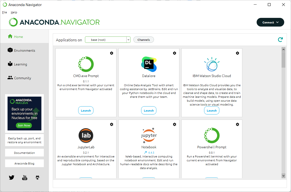
Anaconda Navigator in Windows 11

Anaconda includes easy access to all the tools we’re using in this tutorial, and an absolute ton of other key data science libraries for Python.

One final option is to install and use TensorFlow in Google Colab, which is Google's take on Jupyter notebooks.

The difference being that Colab projects live in Google’s cloud, while Jupyter notebooks in this tutorial will be locally installed and use your machine’s processing capabilities.

If you want to go cloud you can learn more about Colab and TensorFlow in this YouTube video.

Now on to a sample TensorFlow project

Now that we have TensorFlow installed, let's try our sample project. If you want to set-up a virtual environment for your project, do that now before we get started:

virtualenv -p python3.8 venv

If you have a different version of virtualenv then you'd substitute your version for python 3.8.

Then when that's done type:

source venv/bin/activate

Now let's start up our Jupyter notebook:

jupyter lab

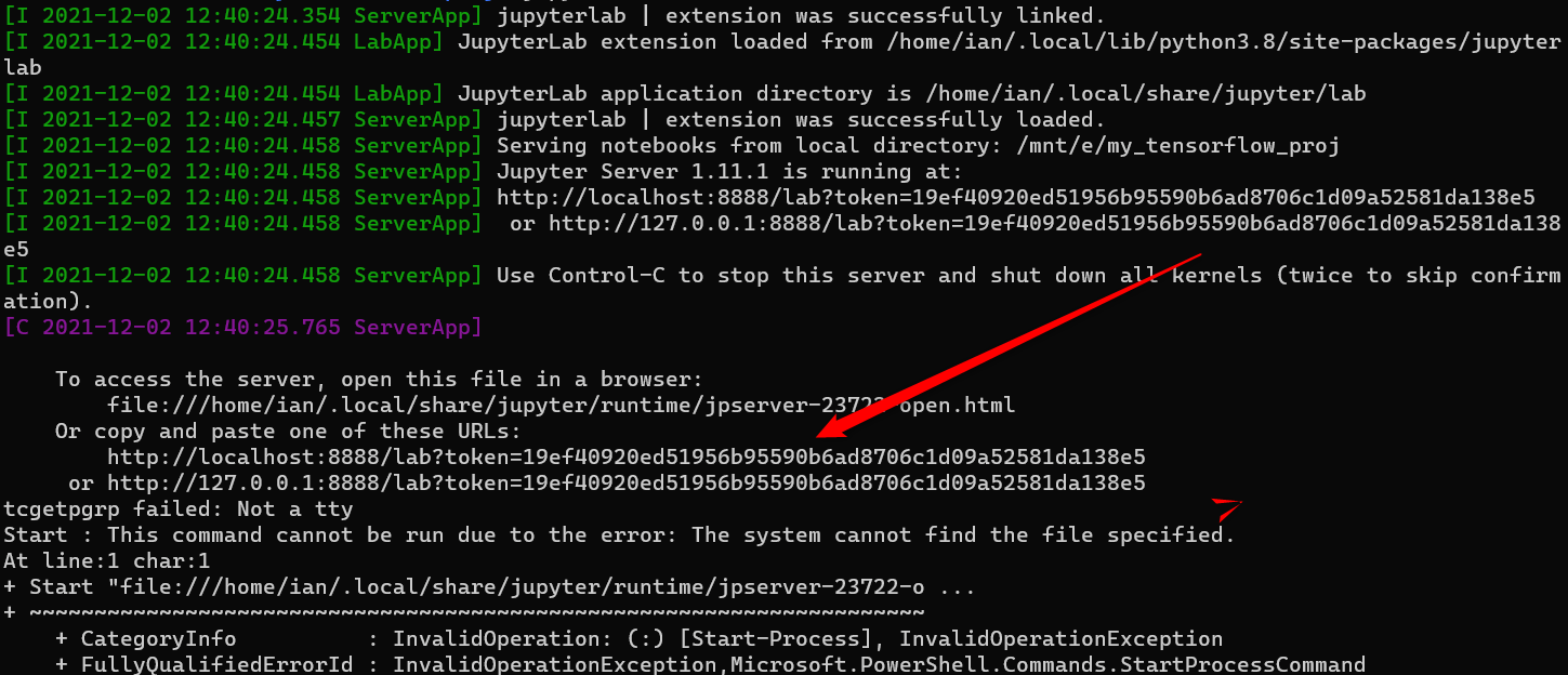
Use a URL like the one the red arrow is pointing to in this image.

After Jupyter starts up, press Ctrl on your keyboard and then click on the "localhost" link shown in your command line, which will open the Jupyter notebook in your default browser.

Next, click on the Python icon under "Notebook" and let's get coding.

Setting up your environment

This sample project isn’t going to break new ground. We’re just going to use the basic image classification tutorial on the TensorFlow website.

Even though we've installed TensorFlow and the other Python libraries on our system we still need to import them into our project.

The first thing we do is import our libraries. Start by typing this into the first cell:

import tensorflow as tf

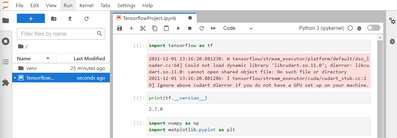
A Jupyter Notebook in Windows 11.

Next click the Play button in the menu above the code cell or hit Shift + Enter on your keyboard.

Doing this makes the code in the cell run. The beauty of Jupyter notebooks is that you can run code in small chunks instead of debugging an entire script after it's written.

In this tutorial each code snippet you see here is meant to be typed into its own cell and then run before moving on.

The first cell is just to make sure TensorFlow is installed and we can import it without issue. If you get an error warning about the GPU don't sweat it. We're not getting into that today and it won't stop our project.

To be doubly sure TensorFlow is ready to go type the following into a new cell and and run it:

print(tf.__version__)

If you get a result then we're all good.

Next, we import our helper libraries:

import numpy as np 
import matplotlib.pyplot as plt

All of our import statements include abbreviations for each library. This is to save time on typing these names inside our project's code. The three abbreviations used here are standard for their respective libraries.

Grab the images

Now we're almost ready to get moving. For this project we're using the Fashion-MNIST dataset from GitHub.

The Keras API allows us to download this dataset directly with the following code:

fashion_pics = tf.keras.datasets.fashion_mnist

You can name the variable whatever you want if "fashion_pics" doesn't grab you. Just make sure you use your variable in the next statement as well.

(train_images, train_labels), (test_images, test_labels) = fashion_pics.load_data()

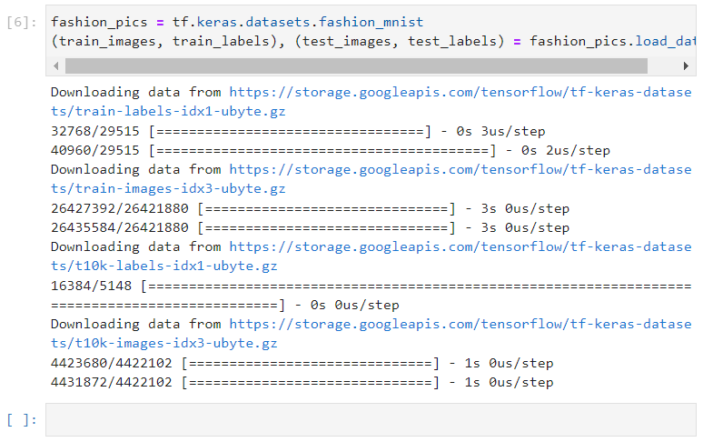
A Jupyter notebook downloading the Fashion-MNIST dataset.

The dataset has 10 labels in total ranging from 0 to 9. Each number represents a type of clothing such as pullover, dress, shirt, and so on. Here's the basic table of the labels and their corresponding descriptions:

Label	Description
0	T-shirt/top
1	Trouser
2	Pullover
3	Dress
4	Coat
5	Sandal
6	Shirt
7	Sneaker
8	Bag
9	Ankle Boot

The dataset doesn’t have the descriptions built-in so let's set-up a list to contain them:

class_names = ['T-shirt/top', 'Trouser', 'Pullover', 'Dress', 'Coat', 'Sandal', 'Shirt', 'Sneaker', 'Bag', 'Ankle boot']

Next, we have to preprocess the data so that we have normalized values between 0 and 1. To do that use the following code:

train_images = train_images / 255.0

test_images = test_images / 255.0

Then it's recommended to create a grid of images to make sure all your labels are behaving as expected:

plt.figure(figsize=(10,10)) 
for i in range(25):     
    plt.subplot(5,5,i+1)     
    plt.xticks([])     
    plt.yticks([])     
    plt.grid(False)     
    plt.imshow(train_images[i], cmap=plt.cm.binary)    plt.xlabel(class_names[train_labels[i]]) 
plt.show()

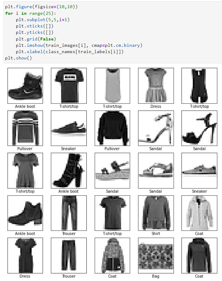
The resulting grid of images looks good.

Build the layers

Now it's time to get down to business by creating those layers that will do all the serious machine learning:

model = tf.keras.Sequential([
    tf.keras.layers.Flatten(input_shape=(28, 28)),
    tf.keras.layers.Dense(128, activation='relu'),
    tf.keras.layers.Dense(10)
])

Next we have to compile the model, which will do a variety of things such as check how accurate the model is during training, update the model based on its training, and other key functions:

model.compile(optimizer='adam', loss=tf.keras.losses.SparseCategoricalCrossentropy(from_logits=True), metrics=['accuracy'])

Now, for the easy part: We let the model do its training:

model.fit(train_images, train_labels, epochs=10)

This will take a little bit of time to work depending on how powerful your machine is, but it shouldn't take longer than a minute or two.

Checking model accuracy

Once the training is done let's check to see how accurate the model is:

test_loss, test_acc = model.evaluate(test_images,  test_labels, verbose=2)
 
print('\nTest accuracy:', test_acc)

This spits out some statistics as seen above. In this example, the model appears to have pretty even results for both training and test data, though according to the TensorFlow tutorial this is still not close enough and means the model has a small amount of overfitting.

That means the model got too exact and paid too close attention to details it shouldn't have, and may not do well with data outside of the dataset.

Would a higher number of epochs improve this result? Let’s find out. We ran the training epochs again this time for 100 epochs to see if we got a different number.

After all that, the accuracy results stayed pretty much the same. If we were working on a production model then it'd probably be back to the drawing board at this point, but for a quick test and familiarization with TensorFlow it's fine.

Making predictions

Next we have to start making some predictions. First, let's create outputs with numbers we can more easily understand.

probability_model = tf.keras.Sequential([model, tf.keras.layers.Softmax()])

Then let's create a variable and make some predictions:

predictions = probability_model.predict(test_images)

Now let's see how it did with predicting the label for a specific image:

predictions[11]

This tells the model to show its prediction for image number 11. Our output is an array with a bunch of numbers. The result shows how confident the model is for each of the 10 categories the image could belong to.

That's not all that helpful for us, though. We want to know the category the model has the highest confidence in as that's the model's actual "choice:"

np.argmax(predictions[11])

Argmax returns the category with the highest confidence, which is 5 or a sandal in this case.

Let's double check this using our labels:

test_labels[11]

Running this in our example the model was right returning a 5 from both the prediction and the label. The model appears to be working. Let's do one more test:

img = test_images[99] 
img = (np.expand_dims(img,0))
single_pred = probability_model.predict(img)

np.argmax(single_pred[0])

Now let's see if we were right:

Test_labels[99]

Again, we got the same number (2 or a pullover in this case). Excellent! We're done.

We've got a working model that shows TensorFlow is up and running. Now it's time to take the next step with our own projects or some more experimentation using tutorials on the TensorFlow website.

Feel free to contact us if you have any questions or take a look at our Deep Learning Solutions if you're interested in a workstation or server to run TensorFlow on.

---

License for the code used in this tutorial:

# MIT License

#

# Copyright (c) 2017 François Chollet

#

# Permission is hereby granted, free of charge, to any person obtaining a

# copy of this software and associated documentation files (the "Software"),

# to deal in the Software without restriction, including without limitation

# the rights to use, copy, modify, merge, publish, distribute, sublicense,

# and/or sell copies of the Software, and to permit persons to whom the

# Software is furnished to do so, subject to the following conditions:

#

# The above copyright notice and this permission notice shall be included in

# all copies or substantial portions of the Software.

#

# THE SOFTWARE IS PROVIDED "AS IS", WITHOUT WARRANTY OF ANY KIND, EXPRESS OR

# IMPLIED, INCLUDING BUT NOT LIMITED TO THE WARRANTIES OF MERCHANTABILITY,

# FITNESS FOR A PARTICULAR PURPOSE AND NONINFRINGEMENT. IN NO EVENT SHALL

# THE AUTHORS OR COPYRIGHT HOLDERS BE LIABLE FOR ANY CLAIM, DAMAGES OR OTHER

# LIABILITY, WHETHER IN AN ACTION OF CONTRACT, TORT OR OTHERWISE, ARISING

# FROM, OUT OF OR IN CONNECTION WITH THE SOFTWARE OR THE USE OR OTHER

# DEALINGS IN THE SOFTWARE.